The world is electrifying at an unprecedented pace, and lithium-ion batteries are the driving force behind this transformation. These energy storage powerhouses fuel our electric vehicles, capture renewable energy sources, and keep our portable devices humming. However, to fully unlock their potential and accelerate the transition to a sustainable future, we must delve deeper into their behavior – understanding their aging processes, performance under varying conditions, and ultimately, how to extend their lifespan.

My research journey from 2018 to 2021 involved extensive analysis of lithium-ion battery data alongside other electrochemical data. During that time, a major challenge was the reliance on proprietary software and workstation-bound analysis, hindering both portability and automation. This limitation often led to frustrating inefficiencies. However, the discovery of Python as a powerful tool for data analysis revolutionized my workflow, bringing greater flexibility and efficiency.

Battery data analysis is a crucial area of research, directly impacting the design of Battery Management Systems (BMS) and, ultimately, the safety of devices powered by these batteries. Unfortunately, beginner-friendly or electrochemist-centric data analysis tools are scarcely available for such investigations. Furthermore, the limited availability of open battery datasets poses a challenge to the development and validation of such tools.

This blog post embarks on an exciting expedition into the realm of battery data analysis, utilizing a valuable resource from the Oxford Battery Degradation Dataset. We will unlock the secrets hidden within this data using Python, exploring key metrics such as capacity fade, state of charge (SOC), and the fascinating insights revealed through dQ/dV analysis.

The Oxford Battery Degradation Dataset

The Oxford Battery Degradation Dataset is an electrochemical battery cycling data from commercially available 18650-format lithium-ion batteries. This dataset captures the battery’s response to various charge and discharge cycles, offering valuable insights into its performance over time.

The battery cycling was conducted using a Maccor 4200 (Maccor Inc., U.S.A.). The charging process involved a constant current of 1.5 A until the voltage reached 4.2 V, followed by a constant voltage phase until the current decreased to 100 mA. Discharging was performed at a constant current of 4.0 A down to a 2.5 V cutoff. This charge-discharge protocol was repeated for a total of 400 cycles, and all cycling was performed within an environmental chamber maintained at a temperature of 24 °C. Our focus will be on the EIL-MJ1-015 dataset; more details can be found in the original paper.

Setting the Stage

Data Loading

Before we dive into the analysis, let’s set the stage by preparing our data. This involves loading, cleaning, and organizing the dataset for easy exploration. Using the power of Python and libraries like Pandas, we can achieve this efficiently:

# Load the dataset
bat_data = pd.read_csv('/content/drive/MyDrive/Colab Notebooks/Oxford Battery Data Analysis/EIL-MJ1-015.csv', header=0)

# Remove unnecessary rows and reset index
bat_data.drop([0], inplace=True)
bat_data.reset_index(drop=True, inplace=True)

# Convert data to the appropriate type
bat_data = bat_data.astype(dtype='float64')

This dataset is comprised of two main sections. The first four columns provide a summary of the cycling data, while the remaining columns contain the detailed cycling data itself.

Data Preprocessing

Before further analysis, the dataset requires some cleaning and preprocessing. Below is the driver code for separating the dataframe based on the cycle number:

# Function to split a dataframe containing cycle number, potential, and capacity columns into separate DataFrames based on cycle number
# Returns a dictionary with cycle numbers as keys and the corresponding dataframes as values.

def split_by_cycle_number(df):
  cycle_dfs = {}
  for cycle_number, group_df in df.groupby('Cycle Number'):
    cycle_dfs[cycle_number] = group_df.copy()
  return cycle_dfs

Below is the driver code for the separation of charge and discharge cycle:

# Function to separate charge and discharge cycles from a battery cycling dataframe containing capacity, voltage, and cycle number columns
# Returns two separate DataFrames: one containing charge cycles and another containing discharge cycles.

def separate_charge_discharge(df):

  # Identify charging based on two consecutive increasing capacities (may need adjustment)
  is_charging = (df['Cell Potential'].diff() >= -0.001) & (df['Cell Potential'].shift(1).diff() >= -0.001)

  charge_df = df[is_charging]
  discharge_df = df[~is_charging]
  return charge_df, discharge_df

Below is the driver code for separating the charge and discharge based on the cycle number:

# Function to split a dataframe containing cycle number, potential, and capacity columns into separate dictionaries for charge and discharge data within each cycle.
# Returns two separate dictionaries: one containing charge DataFrames for each cycle number and another containing discharge DataFrames for each cycle number.

def separate_charge_discharge_by_cycle(df):
  charge_data = {}
  discharge_data = {}
  for cycle_number, group_df in df.groupby('Cycle Number'):
    charge_df, discharge_df = separate_charge_discharge(group_df.copy())
    charge_data[cycle_number] = charge_df
    discharge_data[cycle_number] = discharge_df
  return charge_data, discharge_data

A detailed analysis using this dataset can be found in the Jupyter notebook available in the associated GitHub repository.

Unveiling Capacity Fade: The Battery’s Aging Secret

One of the most crucial aspects of battery health is capacity fade, which represents the gradual decrease in the battery’s ability to store charge over time. This phenomenon is inevitable, but understanding its progression is key to maximizing battery life.

Using the initial capacity as a baseline, we can calculate capacity fade for each cycle and plot it over time:

# Calculate capacity fade
initial_capacity = bat_summary_df['Discharge Capacity'].iloc[0] 
bat_summary_df['Capacity Fade'] = (initial_capacity - bat_summary_df['Discharge Capacity']) / initial_capacity * 100

# Plot capacity fade over cycles
plt.plot(bat_summary_df['Cycle'], bat_summary_df['Capacity Fade'], marker='o')
plt.xlabel("Cycle Number")
plt.ylabel("Capacity Fade (%)")
plt.title("Capacity Fade over Cycles")
plt.grid(True)
plt.show()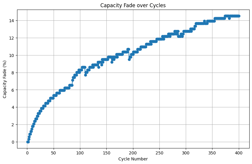

This visualization allows us to track the battery’s capacity decline and identify any potential anomalies or accelerated degradation patterns. In the present example, the battery capacity faded quite faster by more than 14% by 400 cycles!

A Dynamic Measure of Battery Readiness: State of Charge (SOC)

The state of charge (SOC) indicates the remaining charge in the battery, expressed as a percentage of its maximum capacity. This dynamic metric is crucial for battery management systems, ensuring optimal performance and preventing overcharging or deep discharging.

We can calculate SOC using the discharge capacity and rated capacity using the following formula and the driver code:

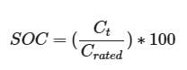
In this formula, C_t represents the battery’s capacity at a specific time (t), while C_rated denotes the maximum rated capacity of the 18650 battery, which is 3.5 Ah.

SOC vs. Cycle Number

By plotting SOC against cycle number, we can visualize how the battery’s capacity to store charge diminishes over repeated cycles. A declining trend in SOC indicates capacity fade, a natural phenomenon in batteries. This information is crucial for predicting battery lifespan and evaluating its long-term performance.

# Calculate SOC
rated_capacity = 3.5 
bat_summary_df['SOC'] = (bat_summary_df['Discharge Capacity'] / rated_capacity) * 100

# Plot SOC over cycles
plt.plot(bat_summary_df['Cycle'], bat_summary_df['SOC'], marker='o')
plt.xlabel("Cycle Number")
plt.ylabel("State of Charge (SOC) (%)")
plt.title("SOC over Cycles")
plt.grid(True)
plt.show()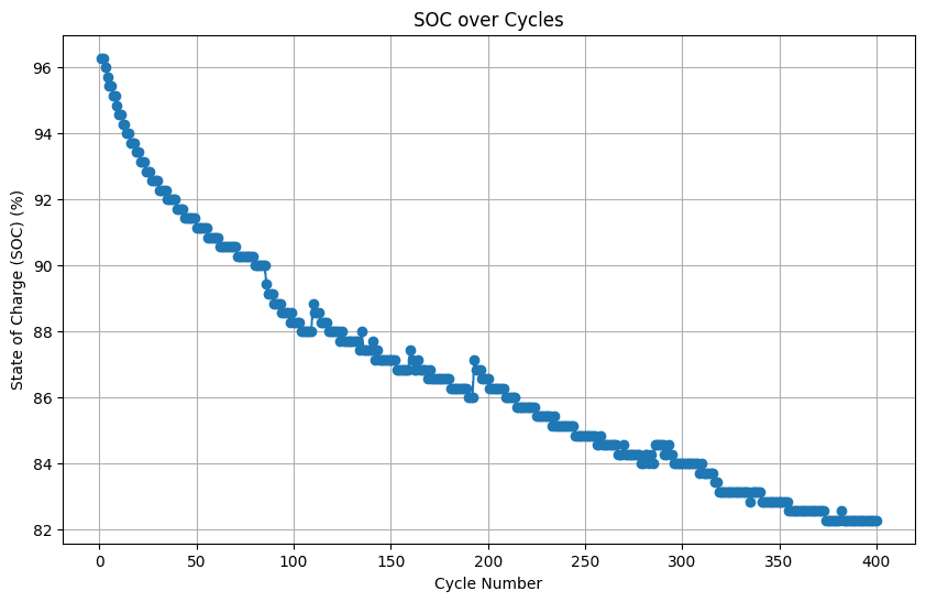

Analyzing SOC vs. cycles helps estimate the battery’s cycle life, which refers to the number of charge- discharge cycles a battery can undergo before its capacity falls below a certain threshold (e.g., 80% of its initial capacity). This information is essential for battery management and replacement planning.

Cell Potential vs. SOC

Cell potential is a direct indicator of the battery’s SOC. By measuring the cell potential, you can estimate the amount of charge remaining in the battery. This is crucial for battery management systems (BMS) to accurately track the battery’s energy level and provide users with reliable information about its remaining runtime.

The shape and slope of the cell potential vs. SOC curve can indicate the battery’s performance characteristics, such as its capacity, energy density, and power output. A steeper slope indicates a higher power capability, while a flatter curve suggests a higher energy density. Analyzing this relationship helps evaluate the battery’s suitability for specific applications.

Changes in the cell potential vs. the SOC curve over time can reveal information about battery degradation. For example, a decrease in the overall potential range or a shift in the curve’s shape can indicate capacity fade or increased internal resistance. Monitoring these changes helps assess battery health and predict its remaining useful life.

Temperature’s Impact on Battery Performance

Battery temperature plays a crucial role in dictating its performance, lifespan, and overall safety. By plotting temperature against cycle number, valuable insights into battery behavior can be obtained. This visualization unveils the temperature fluctuations during charging and discharging cycles, revealing potential issues with the battery’s health and performance.

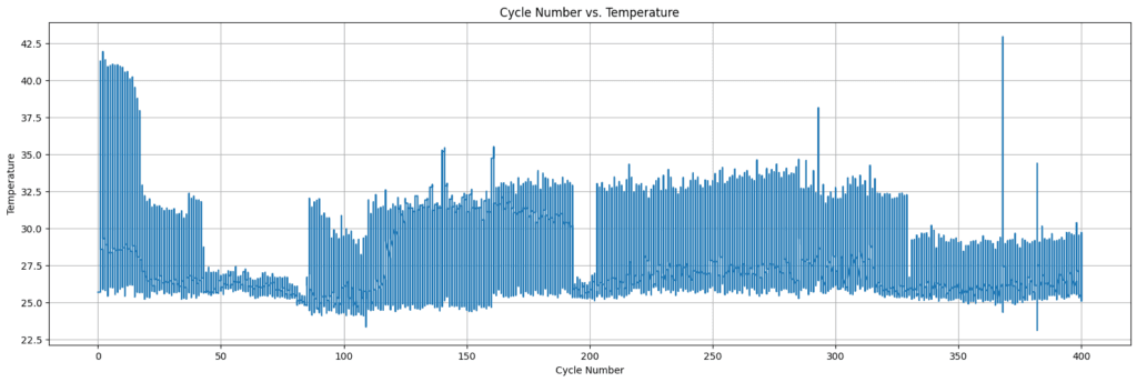
For example, a sharp temperature increase could signal problems with internal resistance or thermal management, crucial factors influencing battery degradation. Continuously monitoring battery temperature through these plots aids in the early detection of potential issues, enabling proactive measures to prevent further damage and maximize battery lifespan. Ultimately, understanding the temperature vs. cycle number plot is essential for researchers and engineers to optimize battery operation, enhance longevity, and ensure safety.

Decoding dQ/dV: Unveiling Electrochemical Signatures

The differential capacity analysis (dQ/dV) is a powerful technique that reveals subtle electrochemical processes within the battery. By plotting dQ/dV against cell potential, we can identify characteristic peaks and valleys that correspond to specific reactions during charge and discharge.

# Calculate dQ/dV
discharge_df['dQ/dV'] = np.gradient(discharge_df['Capacity'], discharge_df['Cell Potential'])

# Plot dQ/dV against cell potential for selected cycles
cycles_to_plot = [1.0, 2.0, 3.0, 4.0, 5.0]
for cycle in cycles_to_plot:
    cycle_df = discharge_df[discharge_df['Cycle Number'] == cycle]
    plt.plot(cycle_df['Cell Potential'], cycle_df['dQ/dV'], label=f'Cycle {int(cycle)}')

plt.xlabel('Cell Potential (V)')
plt.ylabel('dQ/dV (Ah/V)')
plt.title('Cell Potential vs. dQ/dV for Selected Discharge Cycles')
plt.legend()
plt.grid(True)
plt.show()

This allows researchers to identify and analyze specific electrochemical reactions, such as phase transitions and solid solution reactions, that take place within the battery’s electrodes. Furthermore, peaks in the dQ/dV curve correspond to specific electrochemical reactions, providing a “fingerprint” of the battery’s behavior.

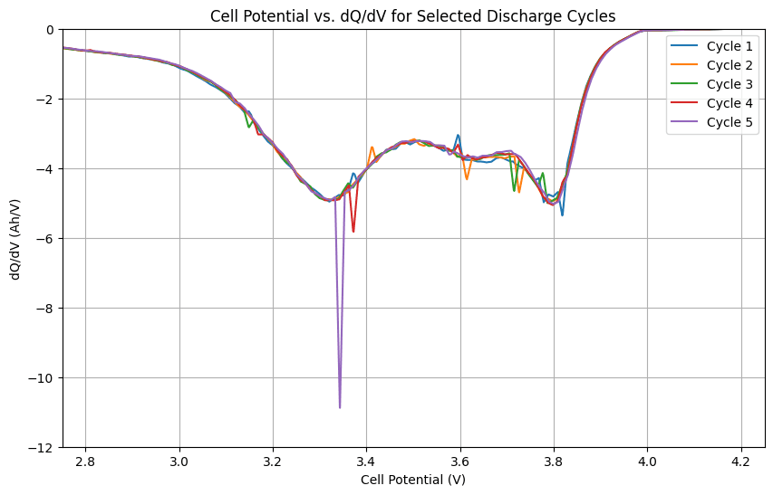
By tracking changes in the dQ/dV curve over time, researchers can monitor the degradation of battery materials and identify the underlying causes of capacity fade and performance loss. Moreover, changes in the position, height, and shape of peaks in the dQ/dV curve can indicate various degradation mechanisms, such as loss of active material, electrolyte decomposition, change in the electrode structure, and increasing internal resistance.

Conclusion

With the growing demand for energy storage solutions, analyzing and interpreting battery data is increasingly important. The Oxford Battery Data Analysis demonstrates the power of data in understanding battery behavior. Analyzing metrics like capacity fade, SOC, and dQ/dV provides valuable insights into battery health, performance, and degradation. Additionally, this analysis offers budding electrochemists a unique opportunity to connect theoretical knowledge with practical application.

Data Source and Inspiration

This blog post reproduces some parts of the data analysis presented in the following research article:

• Authors: T. M. M. Heenan, A. Jnawali, M. D. R. Kok, T. G Tranter, C. Tan, A. Dimitrijevic, R. Jervis, D. J. L. Brett, and P. R. Shearing
• Title: An Advanced Microstructural and Electrochemical Datasheet on 18650 Li-Ion Batteries with Nickel-Rich NMC811 Cathodes and Graphite-Silicon Anodes
• Journal: Journal of The Electrochemical Society
• DOI: 10.1149/1945-7111/abc4c1

This blog post would not have been possible without the foundational work of the original authors, whose contributions are gratefully acknowledged

Citation

If you use the code from this post, please cite it as follows: Battery Data Analysis, Aravindan Natarajan, https://github.com/anatarajank/Battery-Data-Analysis